R Package to Calculate Income Taxes

A joy of programming is making tools to solve your everyday problems. For example, I found myself often having to estimate income taxes on various economic data sets that included income and family characteristics. I felt like I was starting fresh each time: figuring out what external tool to use; cleaning the data to put it in the right format for that tool; and uploading and downloading the results.
Each time, I began by searching for an R package that automatically calculates income taxes. And each search came up empty. So, I build the package myself.
usincometaxes calculates federal and state income taxes, all within R. Technically, the package doesn’t calculate the taxes. It relies on the NBER’s TAXSIM35 tax calculator to do the hard work.
usincometaxes gets the data in the right format, performs checks on the data to ensure the format is correct, sends the data to TAXSIM35’s server, and pulls the data back into an R data frame. The user simply has to call a function to calculate taxes and wait for the results to fall into an R data frame.
usincometaxes’s documentation contains instructions and vignettes. But, here is a quick example to wet your appetite.
Example of using usincometaxes
usincometaxes contains a dataset with simulated income and household data that we will use to calculate taxes.
library(usincometaxes)
library(gt)
library(tidyverse)
data(taxpayer_finances)
head(taxpayer_finances) %>%
head() %>%
gt()| taxsimid | year | mstat | state | page | sage | depx | age1 | age2 | age3 | pwages | swages | dividends | intrec | stcg | ltcg |
|---|---|---|---|---|---|---|---|---|---|---|---|---|---|---|---|
| 1 | 2000 | single | NC | 37 | 0 | 4 | 6 | 7 | 8 | 26361.75 | 0.00 | 2260.86 | 4340.19 | 2280.16 | 2060.29 |
| 2 | 2000 | single | NC | 29 | 0 | 1 | 7 | 0 | 0 | 33966.34 | 0.00 | 1969.54 | 868.10 | 1064.50 | 2234.61 |
| 3 | 2000 | married, jointly | NC | 36 | 30 | 1 | 13 | 0 | 0 | 174191.53 | 102286.98 | 1972.47 | 2048.31 | 1009.11 | 1226.34 |
| 4 | 2000 | married, jointly | NC | 37 | 34 | 3 | 5 | 6 | 7 | 67604.57 | 53205.76 | 1173.95 | 881.67 | 3582.74 | 1405.74 |
| 5 | 2000 | married, jointly | NC | 38 | 39 | 0 | 0 | 0 | 0 | 21176.78 | 21687.72 | 4614.91 | 1588.52 | 560.93 | 825.04 |
| 6 | 2000 | single | NC | 36 | 0 | 1 | 2 | 0 | 0 | 53397.72 | 0.00 | 2067.41 | 1320.01 | 687.23 | 3548.07 |
Now, let’s calculate federal and state income taxes.
family_taxes <- taxsim_calculate_taxes(
  .data = taxpayer_finances,
  return_all_information = FALSE
)
family_taxes %>%
  head() %>%
gt()| taxsimid | fiitax | siitax | fica | frate | srate | ficar | tfica |
|---|---|---|---|---|---|---|---|
| 1 | 924.97 | 1046.23 | 4033.35 | 15.00 | 7.00 | 15.3 | 2016.67 |
| 2 | 3596.23 | 1947.22 | 5196.85 | 15.00 | 7.00 | 15.3 | 2598.42 |
| 3 | 78080.32 | 20429.27 | 26915.48 | 36.58 | 8.12 | 2.9 | 13457.74 |
| 4 | 23279.56 | 7783.72 | 18483.98 | 30.83 | 7.75 | 15.3 | 9241.99 |
| 5 | 5584.33 | 2619.27 | 6558.27 | 15.00 | 7.00 | 15.3 | 3279.13 |
| 6 | 8358.38 | 3411.43 | 8169.85 | 28.00 | 7.00 | 15.3 | 4084.93 |
The column fiitax is federal income taxes and siitax is state income taxes. See the description of output columns vignette for more information on the output columns.
Let’s combine our income tax dataset with the original dataset containing household characteristics and income.
income_and_taxes <- taxpayer_finances %>%
  left_join(family_taxes, by = 'taxsimid')
Now we have a single data frame containing both wages and income tax liabilities. Let’s take a look at the relationship between wages and estimated federal income taxes. The colors represent the number of children 18 or younger.
# custom theme for all plots in the vignette
plt_theme <- function() {

    theme_minimal() +
    theme(
      legend.text = element_text(size = 11),
      axis.text = element_text(size = 10),
      axis.title=element_text(size=11,face="bold"),
      strip.text = element_text(size = 11),
      panel.grid.minor = element_blank(),
      plot.title = element_text(face = "bold"),
      plot.subtitle = element_text(size = 12),
      legend.position = 'bottom'
    )
}

# color palettes for number of children
dep_color_palette <- rev(c('#4B0055','#353E7C','#007094','#009B95','#00BE7D','#96D84B'))
income_and_taxes %>%
  mutate(
    tax_unit_income = pwages + swages,
    num_dependents_eitc = factor(depx, levels = as.character(0:5)),
    filing_status = tools::toTitleCase(mstat)
  ) %>%
  ggplot(aes(tax_unit_income, fiitax, color = num_dependents_eitc)) +
    geom_point(alpha = .5) +
    scale_x_continuous(labels = scales::label_dollar(scale = .001, suffix = "K"), limits = c(0, 200000)) +
    scale_y_continuous(labels = scales::label_dollar(scale = .001, suffix = "K"), limits = c(-10000, 50000)) +
    scale_color_discrete(type = dep_color_palette) +
    facet_grid(rows = vars(mstat), cols = vars(year)) +
    labs(
      title = "Federal Income Taxes by Filing Status, Year, and Number of Children",
      x = "\nHousehold Wages",
      y = "Federal Income Taxes"
    ) +
    plt_theme() +
    guides(color = guide_legend(title = "Number of Childern 18 or Younger", title.position = "top", byrow = TRUE))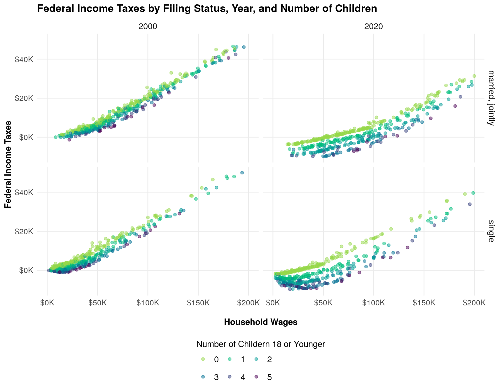
And that’s all there is to it.
As mentioned earlier, the TAXSIM35 tax calculator does all the hard work of calculating taxes. So, if you use usincometaxes in your work, please cite TAXSIM:
Links
usincometaxesdocumentationusincometaxeson GitHub- TAXSIM35 tax calculator, which conducts all the tax calculations.
Shane Orr
Education Analyst
Spent six years playing Army, another three as a lawyer, and finally settled into being a data and programming guy.