Bayesian Bar Passage: A Tutorial on Bayesian Hierarchical Modeling in R

What are hierarchical models?

First, let’s load and clean our bar passage data.

library(knitr)
library(rstanarm)
library(tidybayes)
library(glue)
library(tidyverse)
library(ggridges)

# stan options
# detect and use max number of cores
options(mc.cores = parallel::detectCores())

# Data import and cleaning -----------------------------

# all the ABA datasets are on GitHub
# we will save the directory to the repo, for less typing
data_dir <- 'https://raw.githubusercontent.com/shanejorr/ABA-509-disclosures/main/data/'

#import bar passage for all schools data set
bar <- read_csv(glue("{data_dir}First-Time_Bar_Passage_(Jurisdiction-Level).csv")) %>%
  select(-schoolid, -calendaryear) %>%
  # rename year column for easier future reference
  rename(year = firsttimebaryear) %>%
  # only keep 2014 and later
  # our admissions data starts at class entering in 2011, which is 2014 bar year,
  # so 2014 is the earliest bar exam year we can use
  filter(year >= 2014)

#import admissions data so we can extract a school's UPGA and LSAT
admiss <- read_csv(glue("{data_dir}Admissions.csv"))  %>%
  select(schoolname, calendaryear, uggpa75, uggpa50, uggpa25, lsat75, lsat50, lsat25) %>%
  # large outlier in GPA; remove because school is in PR and its GPA
  # could impact scaling
  filter(!str_detect(schoolname, 'Pontifical'),
         # arizona summit in 2021 seems odd regarding its lsat and GPA, so remove
         !(schoolname == "Arizona Summit Law School" & calendaryear == 2018)) %>%
  # students in these admissions classes will take bar in three years
  # so, add three to year, so it matches the bar year
  mutate(year = calendaryear+3) %>%
  # scale gpa and lsat meterics by converting to mean of 0 and standard deviation of 1
  mutate_at(vars(uggpa75, uggpa50, uggpa25, lsat75, lsat50, lsat25), scale) %>%
  select(-calendaryear)

#combine bar results and admissions datasets
bar <- left_join(bar, admiss, by=c('schoolname', 'year')) %>%
  # all WI graduates are listed as passing the bar, so remove
  filter(state != "WI",
        # extreme outlier
        state != "PR")

# create dataset of each state's cumulative pass rate, by year
state_rates <- bar %>%
  group_by(state) %>%
  summarize(takers = sum(takers),
            passers = sum(passers)) %>%
  mutate(pass_rate = passers / takers) %>%
  ungroup()

# find cumulative US pass rate by year, so it can be added to plots
overall_pass <- state_rates %>%
  summarize(takers = sum(takers),
            passers = sum(passers)) %>%
  mutate(pass_rate = passers / takers) %>%
  ungroup()

We start with a simple question: Which states have the lowest and highest bar passage rates? On the surface, this is simple arithmetic. Just divide the number of bar passers by the number of takers. In a way, that’s all there is to it.

But in another context, it’s trickier. Let’s look at Alaska. In our data - spanning 2014 to 2019 - there are two takers and two passers; a bar passage rate of 100%. Do we assume their bar exam is fluff, and if I took it I would be sure to pass? If a thousand cold souls took it would they all pass?

Framing the issue so highlights what we really want to know. We want to know what we’ll call the hypothetical pass rate with an infinite number of takers. Let’s call this the infinite takers pass rate. In other words, if a gazillion people took the Alaska bar, what percentage would pass? Surely it’s not 100%.

Alas, we can never know this number with certainty. We can, however, estimate this rate, along with a probability distribution of possible values for this rate, with a Bayesian hierarchical model.

The above example highlights the problem, albeit in an extreme form, that hierarchical models are designed to solve. To show how they solve it, let’s look at two extreme ways to estimate a state’s infinite pass rate. First, we can simply say that the state’s estimated infinite pass rate is its real pass rate. We could also create confidence intervals for this rate by sampling from a binomial distribution that only contains the state’s takers and passers.

Let’s call this the no-pooling method since we are not using any information outside the state to estimate the state’s rate. This makes sense on the surface, but the problem is that we are making an estimate based on a limited number of data points: limiting our data to the takers within a state. In a state like Alaska this is a problem because there are only two takers.

At the other extreme, we might assume that the best guess for a state’s infinite takers pass rate is the United States pass rate. This gives us more data since we are using data outside the state to predict the state’s rate. With this approach, Alaska’s estimated pass rate is the US rate of 77%. This approach is called complete pooling because we are lumping all states together.

The benefit of this approach is that it gives us more data. Unfortunately, complete pooling arrives with its own squeaky wheel. States have different bar exams with different levels of difficulty. As a result, we can assume that states will have different infinite takers pass rates.

What if we can combine the best of both approaches? What if we primarily use the state’s own rate, but dip into the US rate to the degree that state data is lacking? This concept is called partial-pooling and it provides the backbone of hierarchical models.

To see how it works, let’s put on our jackets and go back to Alaska. With just two data points, we know almost nothing about it’s infinite takers pass rate. And with this fog of almost-ignorance, our best guess might be the US rate.

But, let’s keep in mind we do have two Alaska test takers and they both passed. This is some evidence. Right? Given this, maybe we move our Alaska estimate a percentage point higher than the US rate? This intuitive thought process encapsulates hierarchical methods.

Partial-pooling works for state pass rates because bar exams share commonalities. Almost all states administer the MBE and it counts as roughly half of the final bar exam score in most states. Importantly, MBE is identical between states. This commonality means that information about one state’s pass rate provides some evidence for what another state’s pass rate might be. The evidence isn’t perfect, however, and that is why we only partially-pool this information.

Hierarchically modeling state bar passage rates

With this intuitive understanding of hierarchical models in mind, let’s start modeling.

The plot below shows the results from a Bayesian hierarchical binomial model. The model is binomial because bar passage takes one of two values: pass or fail. Bar exam state is a group-level predictor and pass / fail is the response. The blue dots are the state’s actual pass rate, while red dots are the estimated pass rates. The red line represents the 90% highest posterior interval (HPI). The HPI is akin to the frequentist’s confidence interval. In fact, the HPI is what most people think a confidence interval means: there is a 90% chance that the true infinite takers pass rates falls within the 90% HPI.

# ----- create bayesian model

# create intercept only Bayesian binomial model
state_intercept <- stan_glmer(cbind(passers, takers - passers) ~ (1 | state),
                              prior_intercept = student_t(1, 2.5, 3),
                              iter = 5000, seed = 145,
                              data = state_rates,
                              family = binomial("logit"))

# create posterior distribution of state pass rate predictions
state_draws <- state_rates['state'] %>%
  # predict bar passage rates for each state
  add_fitted_draws(state_intercept, n = 300, seed = 958) %>%
  # calculate hdi and median value of posterior predictions
  group_by(state) %>%
  median_hdi(.value, .width = .95) %>%
  select(-.width, -.point, -.interval) %>%
  # add the actual state rates to the dataset of posterior predictions
  left_join(state_rates, by = 'state')

# ----- create plot of estimates from model

# colors for custom legend
state_draws_colors <- c("Predicted Pass Rate" = "indianred2",
                        "Actual Pass Rate" = "dodgerblue2")

# create plot of bayesian estimated pass rates, actual rates, and HPI
state_draws %>%
  ggplot(aes(.value, fct_reorder(state, .value), color=names(state_draws_colors)[1])) +
  # add vertical line that is the US pass rate
  geom_vline(xintercept = overall_pass$pass_rate, alpha = .7, linetype = 2) +
  # bayesian predicted pass rate
  geom_point(alpha=.7) + 
  # bayesian 95% HPI
  geom_errorbarh(aes(xmax = .upper, xmin = .lower)) + 
  # real pass rate
  geom_point(aes(x=pass_rate, color=names(state_draws_colors)[2]), alpha=.9, size=1) + 
  # convert x-axis to percentage
  scale_x_continuous(labels = scales::percent, limits = c(.5, 1)) +
  scale_color_manual(values = state_draws_colors) +
  labs(title = "Predicted and Actual Bar Passage Rates by State",
       caption = "Data Source: AccessLex",
       x='Bar passage rate',
       y= NULL,
       color = NULL) +
  theme_minimal() +
  theme(legend.position = "bottom")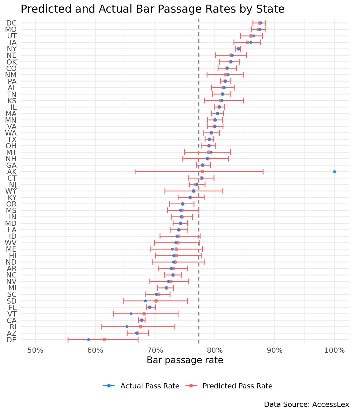

The plot highlights a couple features of Bayesian hierarchical models. First, look at Alaska. Confirming our intuition, the estimated most likely infinite takers pass rate sits a few percentage points higher than the United States rate. Also, Alaska’s wide HPI indicates the lack of data points for the state.

Conversely, look at a state like California that has a lot of bar takers. Its estimated rate is almost identical to its actual rate. When a state has a lot of bar takers, there is less need to infer its estimated state rate from the United States rate. It can infer a pretty exact estimate from the state data alone.

Second, notice that states with actual pass rates higher than the United States average have estimated pass rates lower than their actual rates. And the opposite is true for states with actual pass rates lower than the United States average. This reveals how hierarchical models pull the estimated state rates towards the United States rate. More generically, hierarchical models pull the group estimates towards the global estimate.

Diving deeper: Estimating state passage rates based on LSAT scores and GPA

At this point, our temptation might be to look at the state with the lowest estimated bar passage rate and crown it as having the most difficult bar exam. But, this assumes that states have similar students taking their bar exams. For a host of reasons, this assumption might fail.

We can attempt to control for student quality by incorporating each school’s median undergraduate GPA and LSAT score into the model.

The plot below highlights the correlation between undergraduate GPA, LSAT, and bar passage. The values for GPA and LSAT are normalized to have a mean of zero and standard deviation of one, since this is what we will use for the model. The plot shows that a school’s average GPA and LSAT for its incoming students is positively related to bar passage, so each might be good candidate predictors for our bar passage model.

# create dataset with school pass rate by year, and last and gpa
school_pass <- bar %>%
  group_by(schoolname, year) %>%
  summarize(takers = sum(takers),
            passers = sum(passers),
            lsat = max(lsat50),
            gpa = max(uggpa50)) %>%
  mutate(school_pass = passers / takers) %>%
  select(-takers, -passers)

# create different datasets for lsat and gpa, then we will bind for plotting
lsat <- school_pass %>%
  select(-gpa) %>%
  mutate(type = 'LSAT') %>%
  rename(metric = lsat)

gpa <- school_pass %>%
  select(-lsat) %>%
  mutate(type = 'GPA') %>%
  rename(metric = gpa)

# bind lsat and GPA, and plot as facetted scatterplots
bind_rows(lsat, gpa) %>%
  ggplot(aes(metric, school_pass, color = type)) +
  geom_point(alpha = 0.4, size = 1) +
  facet_wrap(~type, ncol = 1) +
  scale_y_continuous(labels = scales::percent, limits = c(0, 1)) +
  scale_color_brewer(palette = "Set2") +
  labs(title = 'School bar passage rates and student scores',
       x = 'Scaled scores',
       y = 'School bar passage rate') +
  theme_minimal() +
  theme(legend.position="none")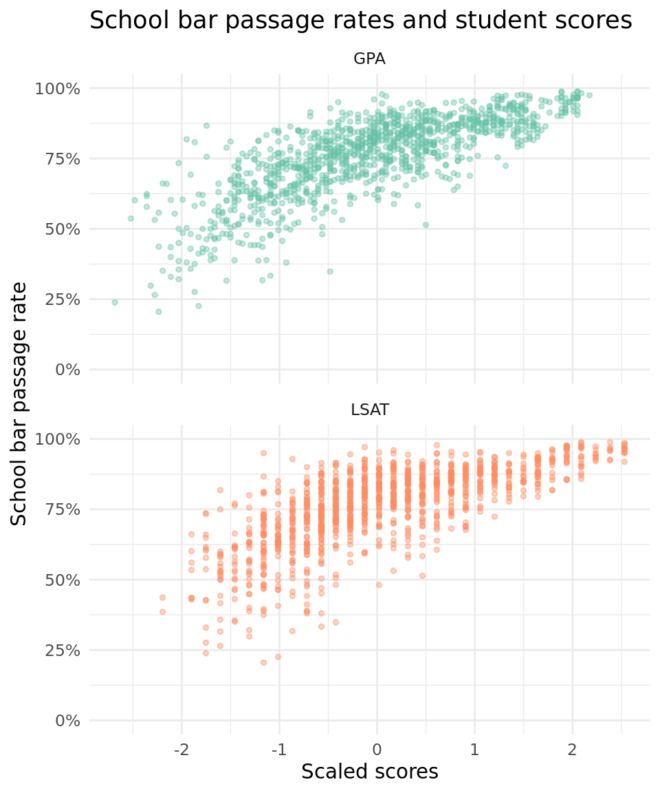

Now, let’s model this relationship by adding the school’s median GPA and LSAT score as additional predictors and keeping state as a group-level predictor.

# create models with GPA and LSAT, test fit, and compare

# only use school / state / year combinations with at least 10 bar takers
# reason: the smaller the number of takers, the less likely that the school's
# mean GPA and LSAT will represent the takers
admissions_mod <- bar %>%
  filter(takers > 10)

# model with state as grouping term, and grades as predictors
# prior intercept is student t, so it is more robust
# prior to regression coefficients is positive, because we have strong prior 
# information that undergrad GPA and LSAT positively relates to bar passage
fit_admissions <- stan_glmer(cbind(passers, takers - passers) ~ uggpa50 + lsat50 + (1 | state),
                            prior_intercept = student_t(1, 2.5, 3),
                            prior = normal(.5, 2.5),
                            iter = 4000, seed = 948,
                            data = admissions_mod,
                            family = binomial("logit"))

# create predictions by predicting passage rates for hypothetical schools in every state
# with mean - 0 - uggpa and LSAT

# get individual states
ind_states <- unique(admissions_mod$state)

admis_mod_pred <- tibble(
  takers = 2000,
  passers = 2000,
  state = ind_states,
  uggpa50 = 0,
  lsat50 = 0) %>%
  # increase number of draws to 1000 since we will plot with ggridges
  add_fitted_draws(fit_admissions, n = 1000, seed = 960) %>%
  ungroup() %>%
  select(state, .value)

The plot below shows the posterior distribution of each state’s predicted bar passage rate with all students hailing from schools that have median LSAT scores and undergraduate GPA. The model attempts to make test-taker ability the same for every state. I say attempts because it is using the school’s median LSAT and undergrad GPA, not the student’s. We show the entire posterior distribution to get a better gauge of uncertainty. These rates should give us a better indicator of bar exam difficulty than the raw pass rate because they attempt to control for student ability.

The posterior distributions also highlight increased uncertainty in low-population states. States with few people have few bar takers and as a result their posterior distributions are flat and wide. On the opposite end, California has a narrow and tall posterior distribution.

ggplot(admis_mod_pred) +  
  # add vertical line that is the US pass rate
  geom_vline(xintercept = overall_pass$pass_rate, alpha = .7, linetype = 2) +
  geom_density_ridges(aes(.value, fct_reorder(state, .value) , group=state), 
                          scale = 3, size = .25, rel_min_height = 0.01,
                      fill = 'dodgerblue2', alpha = .2) +
  scale_x_continuous(labels = scales::percent, limits = c(.5, 1)) +
  labs(title = "Predicted Bar Passage by State",
       subtitle = "Assumes all takers are from schools with median LSAT and undergrad GPA",
       caption = "Data Source: AccessLex",
       x='Bar passage rate',
       y= NULL,
       color = NULL) +
  theme_minimal()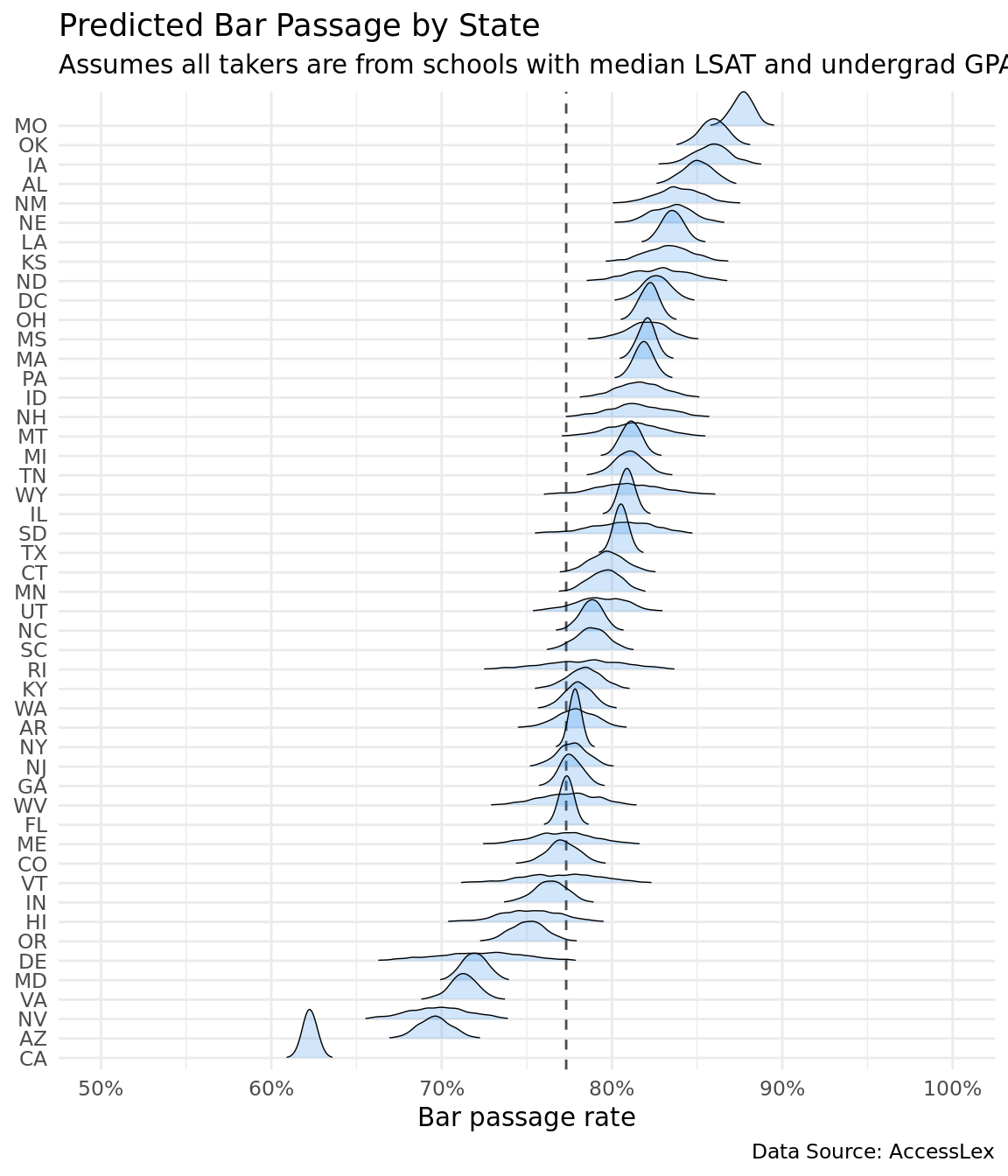

Conclusion

This tutorial provides a 30,000 foot view of Bayesian hierarchical models. They’re great when you have data segmented by groups and those groups share commonalities. In statistics terms, their error terms are correlated. For groups without a lot of data, you can steal information from corollary groups and give yourself more precise estimates with narrower credible intervals.