A First Attempt at Bayesian Mediation Analysis
The same process and ‘almost’ the same results as non-Bayesian approaches, but cooler
What is mediation analysis?
Let’s say you want to examine the affect of employment on whether a student passes a class. You set up a cruel randomized controlled trial where some students are forced to work 15 hours a week and other are prohibited from working at all. You speculate that working students will perform worse because they have less time to study.
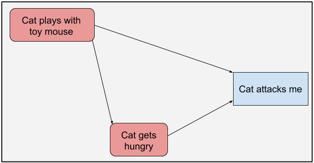
We can visually depict the causal relationships with the following Directed Acyclic Graph (DAG):
knitr::include_graphics(glue::glue("dag/working_dag_main.png"))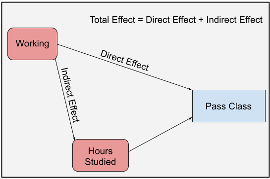
Figure 1: DAG highlighting the effect of working on passing a class
As the graph shows, we might be interested in three different ways that working affects the probability of passing a class.
Direct Effect: The direct effect is the effect that working has on class passage through a direct causal link. There is no intermediate cause between working and passing the class; at least none that we can measure.
Indirect Effect: In our example, working’s indirect effect on bar passage is its effect through hours studied. Working impacts hours studied and hours studied affects class passage.
Total Effect: Total effect is the overall, all things considered, effect of working on passing. It’s the direct effect plus the indirect effect.
The goal of mediation analysis is to disentangle these three effects.
This post is my attempt to manually code a Bayesian mediation analysis. There are packages that do it for you but I could not find one to fit my use case: mediation analysis using a Bayesian logistic regression model and a Bayesian linear regression. So, let’s see if I can do it on my own!
There are a couple different ways to do mediation analysis. This post implements the algorithm explained in the following two papers from Imai et al.
- Unpacking the Black Box of Causality: Learning about Causal Mechanisms from Experimental and Observational Studies
- A General Approach to Causal Mediation Analysis
The appeal of this method is its flexibility. Other methods require models of the same type; for example two Guassian linear models. The method of Imai et al., however, can take any two models as long as they produce predictions. For example, a Guassian linear model and random forest could be used if that’s what your heart desires. This flexibility becomes required if the mediation analysis requires a continuous predictor in one model and a categorical predictor in another. In such a case, you can use a Guassian linear regression and logistic regression. Other methods don’t mix and match so easily.
This post’s wrinkle is that we’re running Bayesian models through the algorithm.
Note: As we’ll see at the end, my results appear a bit off, so I’d advise against blindly following my technique. But, thinking through the issues allowed me to better understand mediation analysis. I hope this post also helps readers deepen their understanding of mediation analysis as well.
Let’s get set up with packages and a series of functions that we will repeatedly use.
library(rstanarm)
library(mediation)
library(tidybayes)
library(glue)
library(knitr)
library(ggeffects)
library(knitr)
library(tidyverse)

# stan options
# detect and use max number of cores
options(mc.cores = parallel::detectCores())

# create ggplot theme for this post
post_theme <- theme_minimal() +
  theme(legend.position = 'bottom',
        plot.title = element_text(size = 10),
        axis.title = element_text(size = 10))

theme_set(post_theme)

# set folder to import pictures
dag_folder <- "content/post/2020-11-25-bayesian-mediation-analysis/dag"
relabel_plot_color <- scale_fill_brewer(palette = "Set2", type = "Qual", labels = c(`0`= "Working", `1` = "Not working"))
posterior_diff <- function(mod, new_df, effect_type) {
# create one column dataframe that is the difference in linear predictions for working and non-working students
# parameters:
# mod: model
# new_df: dataframe to create predictions from
# effect_type: type of effect (indirect, direct, total)
mod_post <- posterior_linpred(mod, newdata = new_df, transform = T,
seed = 1837, n = 500) %>%
as.data.frame()
col_split <- ncol(mod_post)/2
mod_diff <- unlist(mod_post[1:col_split] - mod_post[(col_split+1):ncol(mod_post)])
diff <- data.frame(diff = mod_diff,
type_effect = effect_type)
return(diff)
}
posterior_diff_plot <- function(post_diff, x_limits, plot_title) {
# plot posterior distribution of difference in working and no-working predictions
# parameters:
# post_diff: dataframe created from posterior_diff with predicted posterior
# difference between workers and non-workers
# x_limits: plot x limits
# plot_title: title of plot
ggplot(post_diff, aes(x =diff*100)) +
stat_halfeye(alpha = .7) +
scale_x_continuous(limits = x_limits) +
labs(title = plot_title,
x = 'Perc. point difference in probability of passing class\nNot working - working',
y = 'Density',
fill = NULL)
}
two_group_plot <- function(df, plot_title) {
# plot posterior distribution of both workers and non-workers
# parameters:
# df: dataframe for plotting; will be linear predictions for workers and non-workers
# plot_title: title of plot
ggplot(df, aes(x = .value, fill = as.factor(work))) +
stat_halfeye(alpha = .8) +
scale_x_continuous(labels = scales::percent_format(accuracy = 1)) +
relabel_plot_color +
labs(title = plot_title,
x = 'Probability of passing class',
y = 'Density',
fill = NULL)
}Untangling the Gordian Effects Knot
We’ll simulate a data set to show the three types of effects outlined in the introduction. The fake data set includes three columns: (1) a 0 or 1 identifying whether the student worked with a 1 representing non-working students, (2) a continuous number showing how many hours the student studied in the given week, and (3) a 0 or 1 signifying whether the student passed the class with a 1 showing that the student passed.
# create simulated dataset --------

# number of rows in dataset
n <- 500

# 1 if student does not work, 0 if student works
work_order <- c(1, 0)
working <- rep(work_order, times = n/2)

# save for future use
work_string <- c('Working', 'Not working')

# create vector for hours studied that depends on whether the student worked
set.seed(2938)
study_hours <- rnorm(n,
                     mean = 25 + (working*5),
                     sd = 10)

# create vector for passing the class
# value depends on both hours studied and whether the student worked
final_grade_formula <- (.05 + .015*study_hours + .04*working)
final_grade <- rnorm(n, mean = final_grade_formula, sd = .05)
final_grade <- ifelse(final_grade > 1, 1, final_grade)
final_grade <- ifelse(final_grade < 0, 0, final_grade)
final_grade <- rbinom(n = n, size = 1, prob = final_grade)

grades <- data.frame(
  work = working,
  study = study_hours,
  pass = final_grade
)
Here’s a sample of the data set.
kable(head(grades), digits = 2)| work | study | pass |
|---|---|---|
| 1 | 24.32 | 1 |
| 0 | 27.54 | 1 |
| 1 | 49.45 | 1 |
| 0 | 29.80 | 0 |
| 1 | 33.88 | 0 |
| 0 | 24.95 | 0 |
Direct effect the old fashioned way
In figure 1, the direct effect of working on passing the class is the causal line that does not go through hours studied. TO calculate this effect, we use a single model that predicts passing the class from working status, conditioning on hours studied. By conditioning on hours studied, we block the path from working to class passage that flows through hours studied. This only leaves the direct effect path open.
knitr::include_graphics("dag/working_dag_direct.jpg")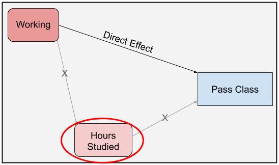
Figure 2: DAG highlighting the direct effect of working on passing a class.
In this situation, we measure the effect of working on class passage, while keeping hours studied the same between workers and non-workers. Converting this idea to a model, we can isolate the direct effect through a simple Bayesian logistic regression model with hours study and working status as predictors and whether the student passed as the response.
# logistic regression model to identify direct effect
full_mod <- stan_glm(pass ~ study + work,
                     family = binomial('logit'),
                     seed = 938,
                     data = grades)
With our model in hand, we can now visualize the direct effect. Figure 3 shows the posterior distribution of the probability of passing the class for both workers and non-workers. The number of hours studied is held constant at the mean number of hours studied: 28.14 hours.
# prediction dataset
mean_hours <- mean(grades$study)

direct_prediction <- data.frame(
  work = work_order,
  study = mean_hours
)

# visualization fo predictions for workers and non-workers
full_mod %>%
  add_fitted_draws(newdata = direct_prediction, seed = 93, n = 300) %>%
  two_group_plot(glue("Prob. of Passing based on Work Status\nHours studied held constant at {round(mean_hours, 2)} Hours"))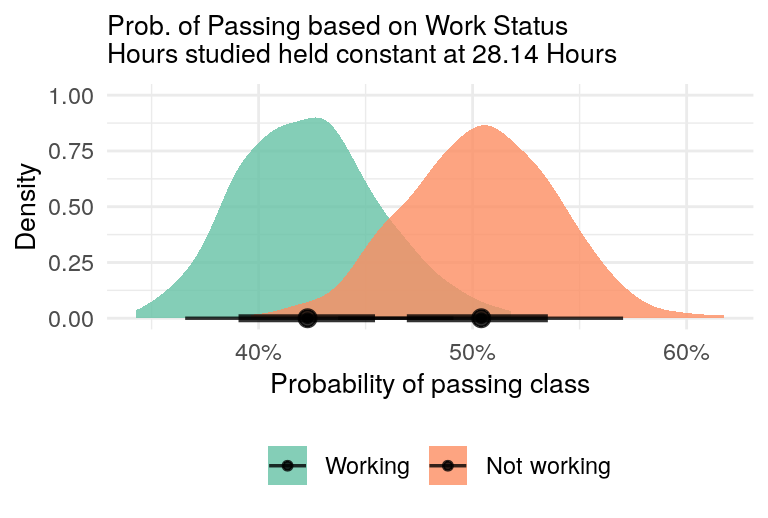
Figure 3: Direct Effect - Difference in class passage probabilities between workers and non-workers, with hours studied held constant.
We see that students who worked have a lower probability of passing the class compared to non-workers, even when accounting for hours studied. But, there is overlap in the probability distributions.
We can better highlight the uncertainty surrounding the difference between workers and non-workers in the probability of passing the class through the following steps:
- Create two posterior predictive distributions for passing the class for each student: one assuming the student worked and another assuming the student did not work.
- For each set of predictions (each student), subtract the posterior predictive distribution arising when the student works from the distribution occurring when the student does not work.
# for each student (observations) create two predictions for passing the class, one if the student worked
# and anotehr if the student did not work

full_mod_newdata <- expand_grid(study = grades$study,
                                work = work_order) %>%
  arrange(desc(work), study) %>%
  as.data.frame()

# find differences in posterior distributions
direct_effect_post <- full_mod %>%
  posterior_diff(new_df = full_mod_newdata, effect_type = 'Direct Effect')
This difference is shown in figure 4. It gives us the posterior predictive distribution of the difference in passing the class between workers and non-workers, holding hours studied constant. It aligns with figure 3, but puts more contours on the magnitude of the difference and its uncertainty.
posterior_diff_plot(direct_effect_post, x_limits = c(-15, 30), plot_title = 'Direct Effect of Working on Passing')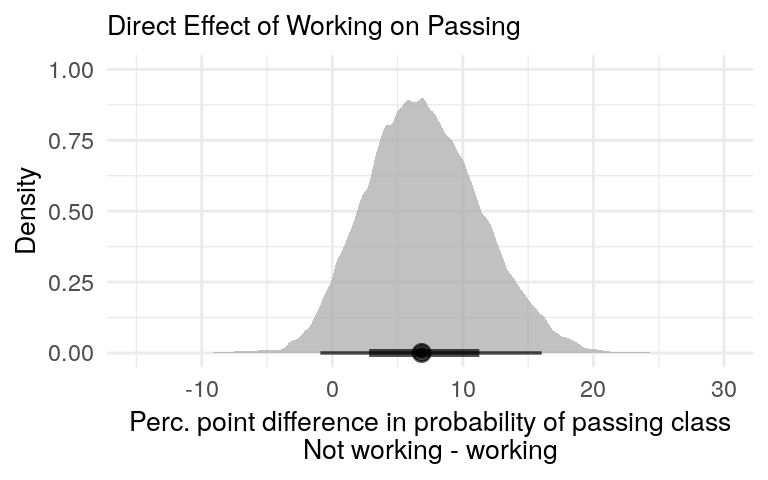
Figure 4: Non-workers are more likely to pass the class.
The posterior distribution of the difference gives us a much better picture of the difference in class passage probabilities between workers and non-workers.
- Direct Effect
- Total Effect
- Indirect Effect
Total effect the old fashioned way
The total effect is the effect of working on class passage through all causal links originating with working. In figure 1, it’s the effect that goes straight from working to class passage combined with the effect that runs through hours studied. We calculate this effect by failing to condition on hours studied. By removing hours studied from the equation, the effect that previously traveled through hours studied now goes directly to class passage. This allows us to merge the two lines into one.
knitr::include_graphics("dag/working_dag_total.png")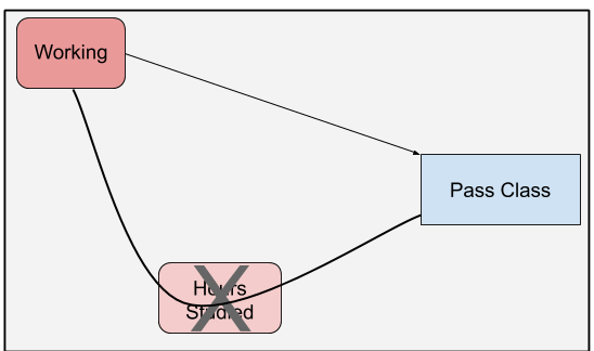
Figure 5: DAG highlighting the effect of working on passing a class
We can estimate the total effect with a Bayesian logistic regression model containing work status as the lone predictor and class passage as the response.
# total effect model
total_effect <- stan_glm(pass ~ work,
                         family = binomial('logit'),
                         seed = 938,
                         data = grades)
As with the direct effect, we can plot the posterior predictive distributions of workers and non-workers.
total_effect %>%
  add_fitted_draws(newdata = data.frame(work = work_order), seed = 93, n = 300) %>%
  two_group_plot('Prob. of Passing based on Work Status')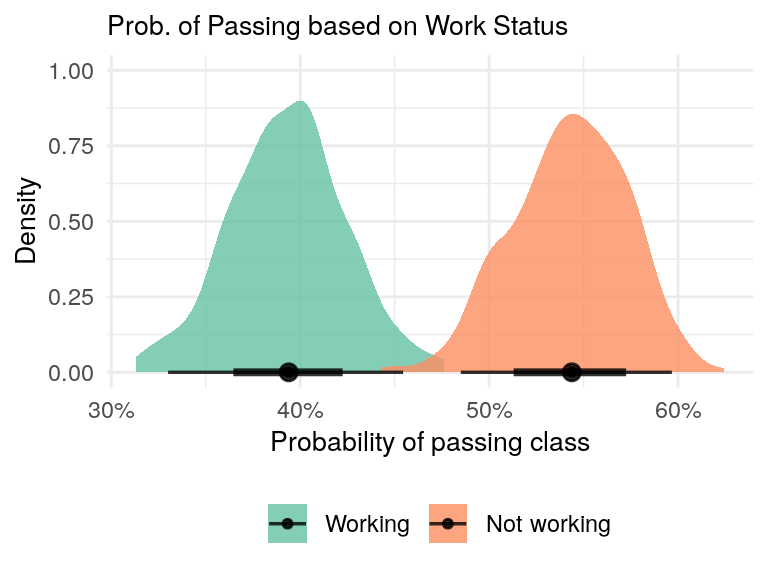
Figure 6: Non-working students have a higher probability of passing the class compared to working students.
We can also focus on the difference and calculate the posterior predictive distribution representing the difference in class passage between workers and non-workers, regardless of hours studied.
diff_limits <- c(-10, 35)

total_effect_post <- total_effect %>%
  posterior_diff(new_df = data.frame(work = work_order), effect_type = 'Total Effect')

posterior_diff_plot(total_effect_post, x_limits = diff_limits, plot_title = 'Total Effect of Working on Passing')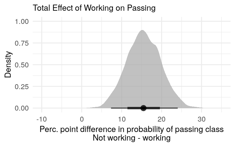
Figure 7: Total effect of working on passing the class. It combines the direct and indirect effects.
The total effect shown in figure 7 is larger than the direct effect from figure 4. This is expected. The total effect includes the direct effect plus effect of studying on passage. Since this later effect is positive, we would expect the total effect to be larger.
Let’s check another item off!.
- Direct Effect
- Total Effect
- Indirect Effect
Indirect effect (kind-of) the old fashioned way
Calculating the indirect effect is more challenging. We want to calculate the effect of working on passing the class that arises because of the effect of working on number of hours studied. Our speculation on the indirect effect is that working causes students to study less, which then leads to them being less likely to pass the class.
Here’s how the authors of the mediation method we’re using describe calculating indirect effect:[^Imai, K., Keele, L., Tingley, D., & Yamamoto, T. (2011). Unpacking the black box of causality: Learning about causal mechanisms from experimental and observational studies. American Political Science Review, 765-789.]
First, we fit regression models for the mediator and outcome. The mediator is modeled as a function of the treatment and any relevant pretreatment covariates. The outcome is modeled as a function of the mediator, the treatment, and the pretreatment covariates. The form of these models is immaterial. … Based on the mediator model, we then generate two sets of predictions for the mediator, one under the treatment and the other under the control.
For the next step, the outcome model is used to make potential outcome predictions. … First, the outcome is predicted under the treatment using the value of the mediator predicted in the treatment condition. Second, the outcome is predicted under the treatment condition but now uses the mediator prediction from the control condition. The ACME [indirect effect] is then computed as the average difference between the outcome predictions using the two different values of the mediator.
Taking our cue from the method’s source, we’ll proceed in two steps: (1) fit models, and (2) make potential outcome predictions.
Step 1: Fitting regression models
The first step is the easiest. We’ll start by fitting two models:
- Mediator model: The mediator (number of hours studied) is the response and the treatment (working status) is the predictor.
- Outcome model: The outcome (passing the class) is the response and the mediator (number of hours studied) and treatment (workign status) as the predictors.
We’ll then create two sets of predictions from the mediator model, one for working students and another for non-working students.
Mediator model
Here is our simple mediator model.
mediator_model <- stan_glm(study ~ work,
                           family = 'gaussian',
                           seed = 938,
                           data = grades)
Outcome model
And here is the almost equally simple outcome model.
outcome_model <- stan_glm(pass ~ work + study,
                          family = binomial('logit'),
                          seed = 938,
                          data = grades)
Predictions from mediator model
Now, we’ll generate predictions from the mediator model. We’ll predict hours studied for both workers and non-workers.
# dataset that only includes two rows, one for a worker and one for a non-worker
mediation_predict_dataset <- data.frame(work = work_order)

mediator_mod_predictions <- add_fitted_draws(newdata = mediation_predict_dataset,
                                             model = mediator_model,
                                             value = 'study',
                                             n = 500,
                                             seed = 1837)
OK, that was easy.
Step 2: Create potential outcome predictions
This is where it get tricky. We want to prediction the outcome - passing the class - using the full outcome model from the predictions created by the mediator model. In essence, we’ll take the predictions about hours studied from the mediator model and use them as the number of hours studied in the full model to create predictions about whether the student passes the class. We’ll assume everyone worked.
Bayesian predictions, however, are not point estimates. They are the full posterior distribution of predicted probabilities. By creating predictions for both workers and non-workers in the mediator model and specifying 500 draws from the posterior distribution - using n = 500 in add_fitted_draws - we now have 1,000 separate predictions of hours studied. 500 for workers and 500 for non-workers. We’ll feed all 1,000 hours studied values to the outcome model and make predictions of passing the class from these 1,000 predictions. Again, all 1,000 values will be assumed to come for workers. I’m sure that sounds convoluted, so here’s the code.
outcome_mod_predictions <- mediator_mod_predictions %>%
  ungroup() %>%
  mutate(mediator_draw = .draw) %>%
  # save the work value from the mediation model because we need to take the difference between the predictions
  # for workers and non-workers as specified in the mediation model
  mutate(work_mediator = work,
         # make all predicted values come from non-workers
         work = 1) %>%
  select(mediator_draw, work_mediator, work, study) %>%
  add_fitted_draws(model = outcome_model,
                   n = 500,
                   seed = 1837) %>%
  ungroup() %>%
  arrange(work_mediator, mediator_draw, .draw, .row)
Finally, we calculate the difference in the probability of passing between workers and non-workers, as labeled in the original mediation model. In calculating the difference, we want to subtract the probability of passing of a non-worker from the probability of a worker. But, which worker and non-worker? There are 500 of each in the mediation model.
For each value in the prediction data set of the outcome model, we stored the work status and sample draw that created the value from the mediation predictions data set. The work_mediator variable distinguishes the workers and non-workers in the mediator model and mediator_draw contains the sample draw from the mediation model. In calculating the difference in probability of passage in the outcome model, we want to pair a worker with a non-worker in the mediation model that has the same sample draw value from the mediation model.
mediation_predictions <- outcome_mod_predictions %>%
  pivot_wider(id_cols = c('mediator_draw', '.draw'),
              names_from = 'work_mediator',
              values_from = '.value') %>%
  rename(worker = `0`, nonworker = `1`) %>%
  mutate(diff = nonworker - worker,
         type_effect = 'Indirect Effect')
All this complete, figure 8 shows the posterior predictive distribution of the indirect effect.
posterior_diff_plot(mediation_predictions, x_limits = c(0, 25), plot_title = 'Indirect Effect of Working on Passing')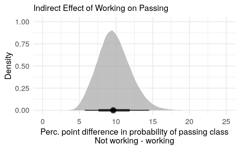
Figure 8: There is a positive indirect effect of not working on passing the class due to the effect of not working on hours studied.
Compare results to mediation package
We did this manually because there is not an R package to automate a mediation analysis when using two different types of Bayesian general linear models. If we had two Gaussian linear models we could streamline the process with the function brm from the brms package. But, I could not get the function to work with a Gaussian and logistic model.
Additionally, the mediation package can be used when mixing Gaussian and logistic models from a frequentest angle. But, we wanted Bayes. However, we can sanity check our results against the mediation package. Our Bayesian models are simple, so the Bayesian and frequentest variants should align.
We’ll first calculate the total, direct, and indirect effects with the mediation package. As you see, it’s a whole lot easier! An entire blog post is encapsulated in six lines of code.
med_fit <- lm(study ~ work, data = grades)

out_fit <- glm(pass ~ work + study,
              data = grades, family = binomial("logit"))

med_out <- mediate(med_fit, out_fit, treat = "work", mediator = "study",
                  robustSE = TRUE, sims = 500)
Now, lets pull out the confidence intervals and point estimates.
# get estimates and conf. intervals for frequentist effect size estimates with mediation package

# dataframe of confidence intervals, with two columns (one for lower and upper bounds)
# will be used for plotting effect sizes
upper_lower_ci <- bind_rows(med_out$z.avg.ci, med_out$d.avg.ci, med_out$tau.ci)

mediation_effects <- tibble(
  effect_type = c('Direct Effect', 'Indirect Effect', 'Total Effect'),
  effect_size = c(med_out$z.avg, med_out$d.avg, med_out$tau.coef),
  lower_ci = upper_lower_ci[[1]],
  upper_ci = upper_lower_ci[[2]],
  effect_group = 'Frequentist (mediation package)'
)
We want to compare the frequentist 95% confidence intervals with our Bayesian 95% credible intervals, which are highest density intervals (hdi). They are not the same, but should be close with our simple models.
# get 95% credible intervals for bayesian effects
bayes_effect <- bind_rows(list(direct_effect_post, mediation_predictions, total_effect_post)) %>%
  group_by(type_effect) %>%
  median_hdi(diff)
Finally, let’s put it all together in one plot.
bayes_effect %>%
  select(effect_type = type_effect, effect_size = diff, lower_ci = .lower, upper_ci = .upper) %>%
  mutate(effect_group = "Bayesian mediation") %>%
  bind_rows(mediation_effects) %>%
    ggplot(aes(effect_size, fct_rev(effect_type), color = effect_group)) +
    geom_point() +
    geom_segment(aes(x = lower_ci, xend = upper_ci, yend = effect_type)) +
    geom_vline(xintercept = 0, alpha = .6) +
    scale_color_brewer(palette = "Set2", type = "Qual") +
    scale_x_continuous(labels = scales::percent_format(accuracy = 1)) +
    facet_wrap(~effect_group, ncol = 1) +
    labs(title = 'Cumulative Effects of Working on Passing Class',
           x = "Percentage point difference (Non-workers minus Workers)\nIn probability of class passage",
           y = NULL) +
    theme(legend.position = 'none')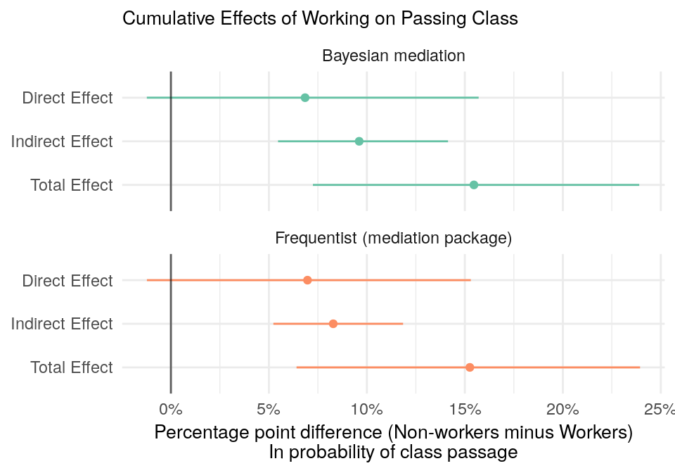
Figure 9: Direct, indirect, and total effects of working on class passage. Values are the average percentage point difference in class passage.
The direct and total effects are almost identical between our homemade Bayesian version and the mediation package. But, these are the easy effects to compute. Let’s not pat ourselves on the back yet. The indirect effects are slightly different. The point estimate of our Bayesian version (I know, real Bayesians don’t use point estimates) is a couple percentage points higher than estimate from the mediation package. Our credible intervals are also larger than the mediation package’s confidence intervals (I know, they’re not the same thing).
It’s hard to know whether the difference is because our homemade version is wrong or because it represents a Bayesian / frequentist difference. My gut tells me that our version is off. The models are too simple for the Bayesian / frequentist difference to matter, as shown by the total and direct effects.
So, you may not want to blindly copy my Bayesian method for mediation analysis. Nonetheless, I hope learned something going through the process.
Shane Orr
Education Analyst
Spent six years playing Army, another three as a lawyer, and finally settled into being a data and programming guy.